Plot and compare model and data

The examples below make use of a numpy ndarray df containing dummy data (you may also use a pandas dataframe), that can be loaded with:

from plothist_utils import get_dummy_data

df = get_dummy_data()

Note

This page presents functions of plothist step by step and gives information about how to use them. To reproduce the examples, please visit the example gallery, because it contains a standalone script for each example, that you can run directly.

Creating the data and model

Below is the code that generates the data and model histograms used in all the examples of this section.

The idea is to have a data_hist corresponding to any kind of data representing a count of entries for a variable, a signal_hist corresponding to the signal model, and a list of background_hists used to model everything that is not the signal. We also define 3 functions that will be used as model components.

We also show an example of how to scale the model to the data. We take advantage that the histograms are separated from the plotting functions to do this, so they can be manipulated before being plotted.

from plothist import make_hist, get_color_palette

key = "variable_1"
range = (-9, 12)
category = "category"

# Define some masks to separate the dataset in signal (1 category), background (3 categories) and data (1 category)
signal_mask = df[category] == 7
data_mask = df[category] == 8

background_categories = [0, 1, 2]
background_categories_labels = [f"c{i}" for i in background_categories]
background_categories_colors = get_color_palette("cubehelix", len(background_categories))

background_masks = [df[category] == p for p in background_categories]

# Create the histograms using the masks defined above
data_hist = make_hist(df[key][data_mask], bins=50, range=range, weights=1)
background_hists = [make_hist(df[key][mask], bins=50, range=range, weights=1) for mask in background_masks]
signal_hist = make_hist(df[key][signal_mask], bins=50, range=range, weights=1)

# Optional: scale to data
# boost_histogram.Histogram objects are easy to manipulate.
# Here, we multiply them by a scalar to scale them, and their variance is correctly scaled as well.
background_scaling_factor = data_hist.sum().value / sum(background_hists).sum().value
background_hists = [background_scaling_factor * h for h in background_hists]

signal_scaling_factor = data_hist.sum().value / signal_hist.sum().value
signal_hist *= signal_scaling_factor


# Define some random functions that will be used as model components with functions
from scipy.stats import norm


def f_signal(x):
    return 1000 * norm.pdf(x, loc=0.5, scale=3)


def f_background1(x):
    return 1000 * norm.pdf(x, loc=-1.5, scale=4)


def f_background2(x):
    return 3000 * norm.pdf(x, loc=-1.8, scale=1.8)

Simple model plots

To only plot the model, the function plot_model() can be used. It supports models made of either functions or histograms. Stacked and unstacked components can be combined. The sum will always be the sum of all the components, stacked and unstacked.

It can take a lot more arguments to customize the plot than shown in the examples below, see the Package references for more details.

Histograms

Here is an example with a model made of 3 stacked and 1 unstacked histograms. The calculated sum is the sum of all 4 histograms.

from plothist import add_text, plot_model

fig, ax = plot_model(
    stacked_components=background_hists,
    stacked_labels=background_categories_labels,
    stacked_colors=background_categories_colors,
    unstacked_components=[signal_hist],
    unstacked_labels=["Signal"],
    unstacked_colors=["black"],
    unstacked_kwargs_list=[{"linestyle": "dotted"}],
    xlabel=key,
    ylabel="Entries",
    model_sum_kwargs={"show": True, "label": "Model", "color": "navy"},
    model_uncertainty_label="Stat. unc.",
)

add_text("Model made of histograms", ax=ax)

fig.savefig(
    "model_with_stacked_and_unstacked_histograms_components.svg",
    bbox_inches="tight",
)

Note

To plot the uncertainty of any histogram as a hashed area, as done automatically in plot_model() for the model, you can use the standalone function plot_hist_uncertainties().

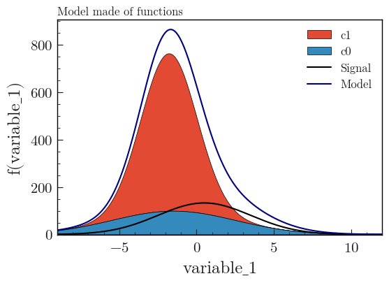
Functions

Here is an example with a model made of 2 stacked and 1 unstacked functions:

from plothist import add_text, plot_model

fig, ax = plot_model(
    stacked_components=[f_background1, f_background2],
    stacked_labels=background_categories_labels[:2],
    unstacked_components=[f_signal],
    unstacked_labels=["Signal"],
    unstacked_colors=["black"],
    xlabel=key,
    ylabel=f"f({key})",
    model_sum_kwargs={"show": True, "label": "Model", "color": "navy"},
    function_range=range,
)

add_text("Model made of functions", ax=ax)

fig.savefig(
    "model_with_stacked_and_unstacked_function_components.svg", bbox_inches="tight"
)

Compare data and model

A data histogram can be added to the plot with plot_data_model_comparison(). It will then compare the sum of the components to the data, with the comparison of your choice. The default comparison is the ratio between the model and the data. It can take any comparison method available in plot_comparison().

The plot_data_model_comparison() is internally a combination of plot_error_hist() for the data, plot_model() for the model, and plot_comparison() for the comparison.

plot_data_model_comparison() can take a lot more arguments to customize the plot than shown in the examples below, see the Package references for more details.

Stacked histograms

A comparison between data and a model composed of 3 stacked histograms. A signal histogram is also plotted, but it doesn’t belong to the model, so it is not taken into account in the comparison.

from plothist import add_luminosity, plot_data_model_comparison, plot_hist

fig, ax_main, ax_comparison = plot_data_model_comparison(
    data_hist=data_hist,
    stacked_components=background_hists,
    stacked_labels=background_categories_labels,
    stacked_colors=background_categories_colors,
    xlabel=key,
    ylabel="Entries",
)

# Signal histogram not part of the model and therefore not included in the comparison
plot_hist(
    signal_hist,
    ax=ax_main,
    color="red",
    label="Signal",
    histtype="step",
)

ax_main.legend()

add_luminosity(
    collaboration="plothist", ax=ax_main, lumi=3, lumi_unit="zb", preliminary=True
)

fig.savefig("model_examples_stacked.svg", bbox_inches="tight")

Warning

For plot_data_model_comparison(), the data_hist has by default asymmetrical error bars. If the provided histogram is weighted, an error is raised and you need to set data_uncertainty_type="symmetrical". More information in Notes on statistics.

Note

The function add_luminosity() is used here to add information on the integrated luminosity used for the data. This is common practice in high energy physics, and this function is provided to make it easy to add this information to the plot. It is a wrapper around add_text().

Unstacked histograms

The same comparison as above, but we represent the model with unstacked histograms:

from plothist import plot_data_model_comparison

fig, ax_main, ax_comparison = plot_data_model_comparison(
    data_hist=data_hist,
    unstacked_components=background_hists,
    unstacked_labels=background_categories_labels,
    unstacked_colors=background_categories_colors,
    xlabel=key,
    ylabel="Entries",
    model_sum_kwargs={"label": "Sum(hists)", "color": "navy"},
    comparison_ylim=[0.5, 1.5],
)

fig.savefig("model_examples_unstacked.svg", bbox_inches="tight")

Stacked and unstacked histograms

Stacked and unstacked histograms can be combined. The sum of the model components is always the sum of all the components, stacked and unstacked. Below is the same comparison as above, but the model is now composed of 2 stacked and 1 unstacked histograms:

from plothist import plot_data_model_comparison

fig, ax_main, ax_comparison = plot_data_model_comparison(
    data_hist=data_hist,
    stacked_components=background_hists[:2],
    stacked_labels=background_categories_labels[:2],
    stacked_colors=background_categories_colors[:2],
    unstacked_components=background_hists[2:],
    unstacked_labels=background_categories_labels[2:],
    unstacked_colors=background_categories_colors[2:],
    xlabel=key,
    ylabel="Entries",
    model_sum_kwargs={"show": True, "label": "Model", "color": "navy"},
    comparison_ylim=(0.5, 1.5),
)

fig.savefig("model_examples_stacked_unstacked.svg", bbox_inches="tight")

Models made of functions

The function plot_data_model_comparison() can also be used to compare data and a model made of functions. The model below is composed of 2 stacked and 1 unstacked functions. All the functions contribute to the model. The sum of the model components is the sum of all the components, stacked and unstacked:

from plothist import plot_data_model_comparison

fig, ax_main, ax_comparison = plot_data_model_comparison(
    data_hist=data_hist,
    stacked_components=[f_background1, f_background2],
    stacked_labels=["c0", "c1"],
    unstacked_components=[f_signal],
    unstacked_labels=["Signal"],
    unstacked_colors=["#8EBA42"],
    xlabel=key,
    ylabel="Entries",
    model_sum_kwargs={"show": True, "label": "Model", "color": "navy"},
    comparison="pull",
)

fig.savefig(
    "ratio_data_vs_model_with_stacked_and_unstacked_function_components.svg",
    bbox_inches="tight",
)

Note

plot_data_model_comparison() can also be used with only one component as the model. To compare a function with a histogram, just put the function in a list in stacked_components (or unstacked_components, it gives the same result in this case) argument and the histogram in the data_hist argument.

Model uncertainty

As said earlier, the comparison function can take any comparison method available in plot_comparison(). To use pulls instead of the ratio to compare the histograms:

from plothist import plot_data_model_comparison

fig, ax_main, ax_comparison = plot_data_model_comparison(
    data_hist=data_hist,
    stacked_components=background_hists,
    stacked_labels=background_categories_labels,
    stacked_colors=background_categories_colors,
    xlabel=rf"${key}\,\,[TeV/c^2]$",
    ylabel="Candidates per 0.42 $TeV/c^2$",
    comparison="pull",
)

fig.savefig("model_examples_pull.svg", bbox_inches="tight")

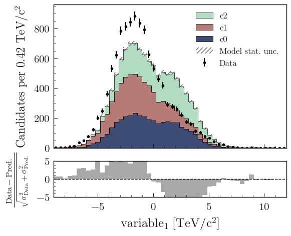
Now, if you do not want to show nor take into account the model uncertainties, setting model_uncertainty to False removes them and updates the definition of the pulls:

from plothist import add_luminosity, plot_data_model_comparison

fig, ax_main, ax_comparison = plot_data_model_comparison(
    data_hist=data_hist,
    stacked_components=background_hists,
    stacked_labels=background_categories_labels,
    stacked_colors=background_categories_colors,
    xlabel=rf"${key}\,\,[eV/c^2]$",
    ylabel=r"Hits in the LMN per $4.2\times 10^{-1}\,\,eV/c^2$",
    comparison="pull",
    model_uncertainty=False,  # <--
)

add_luminosity(collaboration="plothist", ax=ax_main, is_data=False)

fig.savefig("model_examples_pull_no_model_unc.svg", bbox_inches="tight")

The model uncertainties can be removed for every comparison method. Any argument that can be passed to plot_comparison() can be passed to plot_data_model_comparison().

Note

In the two examples above, the bin width is hardcoded in the ylabel. For a 1D histogram with a regular binning, it is possible to get the bin width from the boost_histogram.Histogram object using hist.axes[0].widths[0].

Comparison overview

Here is a collection of examples showing complex plots showing all the possible comparisons between data and model. The idea is to show how to use plot_comparison() and plot_data_model_comparison() to make the plots shown in the examples below. The plots are a bit more complex than the ones shown above, but the code to produce them is still quite simple.

All the different comparisons

Below is shown how to make a plot with all the possible comparisons between data and model. The idea is to use plot_data_model_comparison() to make the plot with the ratio comparison, and then use plot_comparison() to add the other comparisons. The plot_comparison() function can take a fig and ax argument to add the comparison to an existing figure. The plot_data_model_comparison() function returns the figure and axes used to make the plot, so we can use them to add the other comparisons.

from plothist import (
    add_text,
    create_comparison_figure,
    plot_comparison,
    plot_data_model_comparison,
    set_fitting_ylabel_fontsize,
)

fig, axes = create_comparison_figure(
    figsize=(6, 13),
    nrows=6,
    gridspec_kw={"height_ratios": [3, 1, 1, 1, 1, 1]},
    hspace=0.3,
)
background_sum = sum(background_hists)

plot_data_model_comparison(
    data_hist=data_hist,
    stacked_components=background_hists,
    stacked_labels=background_categories_labels,
    stacked_colors=background_categories_colors,
    xlabel="",
    ylabel="Entries",
    comparison="ratio",
    fig=fig,
    ax_main=axes[0],
    ax_comparison=axes[1],
)

add_text(
    r"Multiple data-model comparisons, $\mathbf{with}$ model uncertainty",
    ax=axes[0],
)
add_text(r'  $\mathbf{→}$ comparison = "ratio"', ax=axes[1], fontsize=13)

for k_comp, comparison in enumerate(
    ["split_ratio", "pull", "relative_difference", "difference"], start=2
):
    ax_comparison = axes[k_comp]

    plot_comparison(
        data_hist,
        background_sum,
        ax=ax_comparison,
        comparison=comparison,
        xlabel="",
        h1_label="Data",
        h2_label="Pred.",
        h1_uncertainty_type="asymmetrical",
    )
    add_text(
        rf'  $\mathbf{{→}}$ comparison = "{comparison}"',
        ax=ax_comparison,
        fontsize=13,
    )
    set_fitting_ylabel_fontsize(ax_comparison)

axes[-1].set_xlabel(key)

fig.savefig("model_all_comparisons.svg", bbox_inches="tight")

No model uncertainties

Same example as above, but we remove the statistical uncertainties of the model by adding model_uncertainty=False in plot_data_model_comparison() and pass a model histogram without uncertainties to plot_comparison():

import numpy as np

from plothist import (
    add_text,
    create_comparison_figure,
    plot_comparison,
    plot_data_model_comparison,
    set_fitting_ylabel_fontsize,
)

fig, axes = create_comparison_figure(
    figsize=(6, 13),
    nrows=6,
    gridspec_kw={"height_ratios": [3, 1, 1, 1, 1, 1]},
    hspace=0.3,
)
background_sum = sum(background_hists)

plot_data_model_comparison(
    data_hist=data_hist,
    stacked_components=background_hists,
    stacked_labels=background_categories_labels,
    stacked_colors=background_categories_colors,
    xlabel="",
    ylabel="Entries",
    model_uncertainty=False,  # <--
    comparison="ratio",
    fig=fig,
    ax_main=axes[0],
    ax_comparison=axes[1],
)

add_text(
    r"Multiple data-model comparisons, $\mathbf{without}$ model uncertainty",
    ax=axes[0],
)
add_text(r'  $\mathbf{→}$ comparison = "ratio"', ax=axes[1], fontsize=13)

for k_comp, comparison in enumerate(
    ["split_ratio", "pull", "relative_difference", "difference"], start=2
):
    ax_comparison = axes[k_comp]

    # Copy the original histogram and set the uncertainties of the copy to 0.
    background_sum_copy = background_sum.copy()
    background_sum_copy[:] = np.c_[
        background_sum_copy.values(), np.zeros_like(background_sum_copy.values())
    ]

    plot_comparison(
        data_hist,
        background_sum_copy,
        ax=ax_comparison,
        comparison=comparison,
        xlabel="",
        h1_label="Data",
        h2_label="Pred.",
        h1_uncertainty_type="asymmetrical",
    )
    if comparison == "pull":
        # Since the uncertainties of the model are neglected, the pull label is "(Data - Pred.)/sigma_Data"
        ax_comparison.set_ylabel(r"$\frac{Data-Pred.}{\sigma_{Data}}$")
    add_text(
        rf'  $\mathbf{{→}}$ comparison = "{comparison}"',
        ax=ax_comparison,
        fontsize=13,
    )
    set_fitting_ylabel_fontsize(ax_comparison)

axes[-1].set_xlabel(key)

fig.savefig("model_all_comparisons_no_model_unc.svg", bbox_inches="tight")