Plot result of a fit
This section shows how to plot the result of a fit with pyhf, RooFit or zfit.
pyhf
Here is an example of a fit with pyhf, whose result is then shown using plothist:
import pyhf
import numpy as np
from plothist import make_hist, plot_data_model_comparison

pyhf.set_backend("numpy")

# Define model
data_yield = [100, 50]
model = pyhf.simplemodels.uncorrelated_background(
    signal=[20, 0.0],
    bkg=[75.0, 50.0],
    bkg_uncertainty=[np.sqrt(75.0), np.sqrt(50.0)],
)
data = data_yield + model.config.auxdata
# Maximum likelihood fit
bestfit_pars = pyhf.infer.mle.fit(data, model)
# Extract fit results
model_yields = model.main_model.expected_data(bestfit_pars, return_by_sample=True)

bins = [0, 0.5, 1.0]
data_hist = make_hist(bins=bins)
signal_hist = make_hist(bins=bins)
background_hist = make_hist(bins=bins)

# Set explicitly the content and variance of each bin.
# For the signal and background histograms, we assume no variance.
data_hist[:] = np.c_[data_yield, data_yield]
background_hist[:] = np.c_[model_yields[0], [0.0, 0.0]]
signal_hist[:] = np.c_[model_yields[1], [0.0, 0.0]]

fig, ax_main, ax_comparison = plot_data_model_comparison(
    data_hist=data_hist,
    stacked_components=[background_hist, signal_hist],
    stacked_labels=["Background", "Signal"],
    model_uncertainty=False,
    xlabel="Variable",
    ylabel="Entries",
    comparison="pull",
)
ax_main.set_xticks([0, 0.5, 1.0])
ax_main.tick_params(axis="x", which="minor", bottom=False, top=False)
ax_comparison.set_xticks([0, 0.5, 1.0])
ax_comparison.tick_params(axis="x", which="minor", bottom=False, top=False)

fig.savefig("pyhf.svg", bbox_inches="tight")

In this trivial case, the pulls are null because the model has enough freedom to perfectly fit the two data points.
RooFit or zfit
Two steps are necessary when you want to use plothist to plot the result of a fit using RooFit or zfit.
Getting the PDF
First you need to convert your functions to scipy functions. This can be done using a small function.
With RooFit
This should be called after you have fitted your model and you have a RooAbsPdf object. The idea is to evaluate the RooFit PDF at a large number of points and then interpolate it with a scipy function. This function can then be saved with pickle, or used directly in the following step.
Warning
For a complex PDF that depends on multiple observables, be sure get the correct PDF projection before calling this function. If it doesn’t work, you can use the other method described in Getting RooFit PDFs from the canvas.
import numpy as np
from scipy.interpolate import interp1d
import pickle


def save_pdf(var, pdf, path="pdf.pkl", n_points=10000):
    """
    Save a RooFit PDF as a scipy.interpolate.interp1d function.

    Parameters
    ----------
    var : RooRealVar
       The variable to evaluate the PDF at.
    pdf : RooAbsPdf
       The PDF to save.
    path : str, optional
       The path to save the PDF to. Should end with `.pkl`. Default is "pdf.pkl".
    n_points : int, optional
       The number of points to evaluate the PDF at. Default is 10000.

    Returns
    -------
    pdf_func : scipy.interpolate.interp1d
       The PDF as a function.

    Notes
    -----
    The PDF is saved as a scipy.interpolate.interp1d function with pickle.
    """

    pdf_x = np.zeros(n_points)

    xlim = (var.getMin(), var.getMax())
    # Get a sample of x values
    x = np.linspace(*xlim, n_points)

    for i in range(len(x)):
        var.setVal(x[i])
        # Evaluate the PDF at the given x value
        pdf_x[i] = pdf.getVal(var)

    # Interpolate the PDF
    pdf_func = interp1d(x, pdf_x)

    with open(path, "wb") as f:
        print(f"Saving model to {f.name}")
        pickle.dump(pdf_func, f)

    return pdf_func
With zfit
This should be called after you have fitted your model and you have a zfit.pdf.BasePDF object. The idea is the same as for RooFit: evaluate the PDF at a large number of points and then interpolate it with a scipy function. This function can then be saved with pickle, or used directly in the following step.
from scipy.interpolate import interp1d
import pickle


def save_pdf(var, pdf, path="pdf.pkl", n_points=10000):
    """
    Save a PDF from zfit as a callable function.

    Parameters
    ----------
    var : zfit.Space
        The variable to evaluate the PDF at.
    pdf : zfit.pdf.BasePDF
        The PDF to save.
    path : str, optional
        The path to save the PDF to. Default is "pdf.pkl".
    n_points : int, optional
        The number of points to evaluate the PDF at. Default is 10000.

    Returns
    -------
    pdf_func : scipy.interpolate.interp1d

    Notes
    -----
    The PDF is saved as a scipy.interpolate.interp1d function with pickle.
    """

    lower, upper = var.limits
    x = np.linspace(lower[-1][0], upper[0][0], n_points)

    # Evaluate the PDF at the given points
    pdf_x = zfit.run(pdf.pdf(x, norm_range=var))

    # Interpolate the PDF
    pdf_func = interp1d(x, pdf_x)

    with open(path, "wb") as f:
        print(f"Saving model to {f.name}")
        pickle.dump(pdf_func, f)

    return pdf_func
Renormalize the PDF
A pdf_func you get from a scipy function or from the saved pickle file for RooFit or zfit has an area of 1. When you want to plot it, you need to multiply it by the bin width of your histogram, the number of expected events in the range for this PDF and divide by the integral of the PDF in the range. The small function below performs this renormalization:
from scipy.integrate import quad


def renormalize(pdf, x_range, n_bins, n_data):
    """
    Renormalize a PDF to its corresponding number of data events.

    Parameters
    ----------
    pdf : callable
       The PDF to renormalize.
    x_range : tuple
       The range of the PDF.
    n_bins : int
       The number of bins. Regular binning is assumed.
    n_data : int
       The number of predicted data events in the x_range associated to the pdf.

    Returns
    -------
    pdf : callable
       The renormalized PDF.
    """

    xmin, xmax = x_range
    bin_width = (xmax - xmin) / n_bins
    integral = quad(pdf, xmin, xmax)[0]
    # Note: If x_range is equal to the full range of the PDF, the integral is equal to 1.

    def renormalized_pdf(x):
        return pdf(x) * n_data * bin_width / integral

    return renormalized_pdf
Note
The renormalize function could also be done with a lambda x: function, but it should be use with precautions, see here.
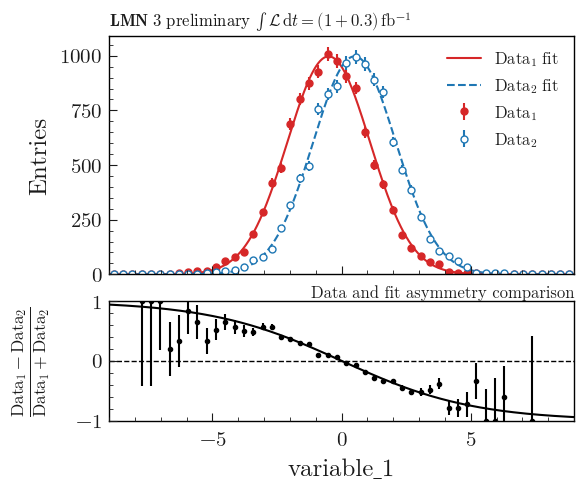
Then you can use plot_model() or plot_data_model_comparison() (see Advanced example using asymmetry comparison) to plot the PDF and do all sort of comparisons with the plothist interface:
Getting RooFit PDFs from the canvas
Some PDFs normalization are not easy to get from the RooFit PDF object.
If the two steps above did not work, you can use the canvas to get the PDF.
This solution has the advantage of being already normalized to the data sample.
The disadvantage is that the resulting PDF is bin dependent, so when plotting your data, you need to use the same bins as the ones used to create the canvas.
To get the PDFs from the canvas, you first need plot the desired PDFs on a frame with plotOn().
Then, you need to save the canvas as a root file with canvas.SaveAs("root_file.root").
The main idea is that when you do a plotOn() on a frame, the function is saved as a TGraph object. You can then get the x and y values of the graph and interpolate it to get a function. The function is then saved in a list with the name of the function. The PDF order in the list is the same as the order you used to plot them on the frame:
import ROOT
from scipy.interpolate import interp1d


def get_pdf_list(root_file_name, canvas_name="canvas"):
    # Open the ROOT file
    root_file = ROOT.TFile(root_file_name, "READ")

    # Get the TCanvas from the file
    canvas = root_file.Get(canvas_name)

    pdf_list = []
    pdf_names = []

    ## If you have multiple pads, you need to specify which one you want to get the PDF from
    # pad = canvas.GetPrimitive("pad_name")
    ## Then loop over the primitives of the pad and not the canvas
    # for obj in pad.GetListOfPrimitives():

    for obj in canvas.GetListOfPrimitives():
        if isinstance(obj, ROOT.TGraph) and not isinstance(obj, ROOT.TGraphAsymmErrors):
            # Get the x and y values of the TGraph
            pdf_names.append(obj.GetName())
            x_values = obj.GetX()
            y_values = obj.GetY()

            # Interpolate the TGraph to get a function
            pdf_func = interp1d(x_values, y_values)

            pdf_list.append(pdf_func)

    print(f"\nPDFs from {root_file_name} saved in the list:")
    for k_name, pdf_name in enumerate(pdf_names):
        print(f"\t[{k_name}] {pdf_name}")
    print()

    return pdf_list